Two curves and  form a wheel-road couple if  can roll without slipping on  so that a fixed point on the plane of  (the wheel hub) has a linear trajectory in the fixed plane. It is therefore a movement of a plane over a fixed plane the base of which is , the rolling curve of which is  and a roulette of which is linear.
The curves  and  can also be considered as two mating gear profiles, the hub of  being located at infinity (consider the movement in a frame linked to the wheel hub).
 

If the wheel  is defined by its polar equation, when its hub is at O, and the road  by its Cartesian equation, the formulas linking the two equations are . From a wheel , we get the road 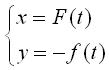 where F is a primitive of fg' (Grégory transformation). Conversely, from a road , we get the wheel 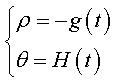 where H is a primitive of . If the wheel is defined by its pedal equation: 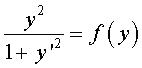, then the differential equation of the road is .

This notion was initially studied, not for a practical use of noncircular wheels, but because the calculations of the curvilinear abscissa are the same for the two curves (for the road, in Cartesian coordinates, and for the wheel, in polar coordinates), so that the rectification of one of them gives that of the other one.
There exist 2 theorems providing a geometrical definition of the road when the wheel is given.
 

1) Steiner-Habich theorem: the road is the roulette with linear base of the negative pedal of the wheel; more precisely, if the negative pedal  of the wheel with respect to the hub rolls on a line, the locus of the hub is the road. In other words: given a curve  and a point, the pedal of this curve with respect to this point and its roulette with linear base form a wheel-road couple.

When (C) rolls on (D), a point M of the plane linked to (C) describes a roulette (R) in the fixed plane. The pedal (P) of (C) with respect to M cuts (D) at the projection M' of M on (D). It can be proved that the curve (P'), symmetrical image of (P) about the perpendicular bisector of [MM'], rolls without slipping on the curve (R), which proves the Habich theorem, since M' describes (D).

2) Mannheim theorem:
Given a curve  and a point, the radial curve of this curve with respect to this point and its Mannheim curve form a wheel-road couple.

Examples:

If the wheel is circular with a centred hub, the road is a line parallel to the trajectory of the hub and it is the only case where this happens, but there is more than just this well-known case!
 

With a circular wheel, but a hub on the boundary, the road is circular; we get the La Hire system. The curve  is a cycloid.
With a circular wheel and a hub anywhere, the curve  is an ellipse or a hyperbola depending on whether the hub is inside or outside the circle, with the hub at a focus; the road is then a roulette of Delaunay.
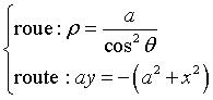
If the wheel is linear (circle with infinite radius), the curve 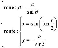 is a parabola with the hub as its focus; the road is a parabolic roulette of Delaunay, in other words, a catenary:. The curve  is a catenary of equal strength.
The case of a linear road not parallel to the trajectory of the hub gives a wheel with the shape of a logarithmic spiral: 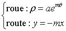.   This property is at the base of the spring-loaded camming device. used for rock climbing.   It could also be used to imagine vehicles with wheels composed of portions of logarithmic spirals rolling on serrated roads.
If the wheel is an Archimedean spiral and the hub its centre, then the road is a parabola: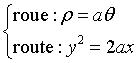. The curves  and  are, here, involutes of circles.
If the wheel is a Fermat spiral and the hub is its centre, then the road is a cubic parabola: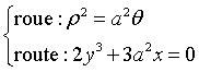
If the wheel is a hyperbolic spiral and the hub is its centre, then the road is a logarithmic curve: .
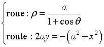
If the wheel is an ellipse and the hub is at one of the foci, then the road is a sinusoid: 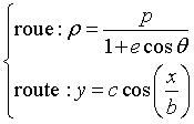 See also the roulette of Delaunay.
If the wheel is an ellipse and the hub is its centre, then the wheel-road couple is: Using the elliptic function of Jacobi dn (JacobiDN in Maple), the equation of the road is 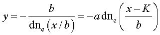 . The curve  is a Talbot curve. See also the Sturm roulette.
If the wheel is a parabola, and the hub its focus, then the road is also a parabola! . The curve  is a Tschirnhausen cubic.
If the wheel is a Kampyle of Eudoxus, and the hub its centre, the road is once again a parabola:  . The curve  is a catenary.
If the wheel is a cardioid and the hub is at its cuspidal point, then the road is a cycloid:. The curve  is then a circle, with the hub on the circle.	Note that the tips of the cycloid have to be slightly trimmed because otherwise they would enter into the wheels at the cuspidal point.
If the wheel is a tractrix spiral and the hub is on its pole, then the road is a tractrix: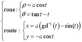 The curve  is a hyperbolic spiral, with the hub at the pole.
If the wheel is a rose and the hub is at the pole, then the road is elliptic 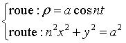; the case n = 1 is none other than the one at the top of this table. The curves  and  are centred cycloids. In the case of a wheel shaped like a conchoid of a rose, the road is a trochoid scaled in one direction. See here the case of the double egg.	Case n = 2
If the road is circular and the hub describes a tangent to the circle, then the wheel is an inverse Norwich spiral. (Remember that if the hub describes a diameter of the circle, then the wheel is circular!)

If the wheel is a sinusoidal spiral with parameter n, then the road is a Ribaucourt curve with parameter 1/n, and the curve  is a sinusoidal spiral with parameter n/(1 – n).

We find several examples given above:
 

n	wheel	road	(G)
-1/2	parabola	parabola	Tschirnhausen cubic
-1	line	catenary	parabola
1/2	cardioid	cycloid	circle
2	lemniscate of Bernoulli	rectangular Sturm roulette	rectangular hyperbola

See also the wheels associated to a Tschirnhausen cubic and, more generally, the wheels associated to pursuit curves.

Compare with the roulettes with linear base.
 

next curve

previous curve

2D curves

3D curves

surfaces

fractals

polyhedra

© Robert FERRÉOL , Alain ESCULIER 2017