Mutual pursuit curves

MUTUAL PURSUIT CURVES (or curves of the n dogs)

Problem posed by Lucas in 1877 in the case of an equilateral triangl [problème des trois chiens, Nouvelles Correspondances Mathématiques 3 p 175-176].
Paper Polygons of pursuit, Bernhart, 1959
Wikipedia: mice problem
Very thorough website in German: did.mat.uni-bayreuth.de/material/verfolgung/node5.html
Animation by G. Tulloue: www.sciences.univ-nantes.fr/sites/genevieve_tulloue/Meca/Cinematique/4mouches.php
Système différentiel de poursuite, Quadrature 129, p. 29, 2023.

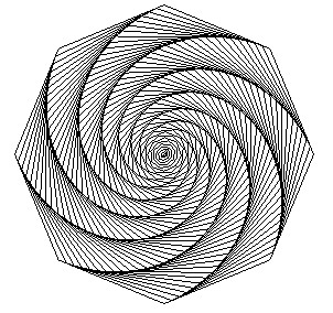
When n points M₁,M₂,…,M_n (traditionally, flies, mice, ladybirds...) chase one another each at the constant speed, with M_k chasing M_k+1 (and M_n chasing M₁), the trajectories of these points are mutual pursuit curves.
The movements and trajectories of the pursuers are then governed by the differential system formed by the n relations .
Note that when is proportional to , the system becomes linear and resolves exactly.

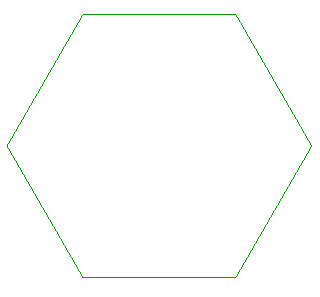
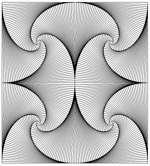
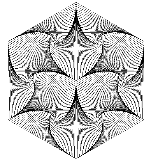
Case of a triangle ABC (A following B, following C, following A)

It can be noted in the particular case below that the two flies that were the furthest apart are the ones who meet first!
It can be shown that the triangle formed by the dogs remains similar to itself if and only if the starting triangle is equilateral.
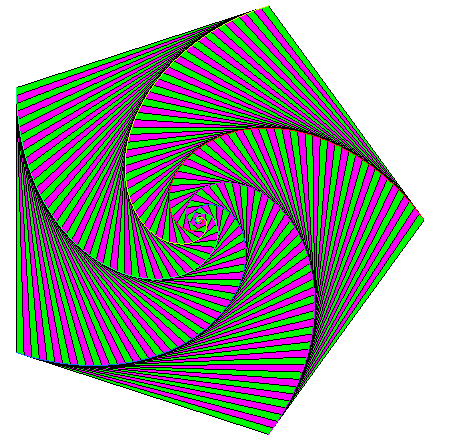
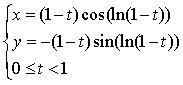
However, if we consider that the dogs can have distinct velocities, then R.K. Miller determined in 1871 that the triangle remains similar to itself if and only if the respective velocities of A,B,C are proportional to (classical notations of the sides of a triangle).
In this case, the first Brocard point of the triangle formed by the dogs remains fixed and the dogs meet simultaneously at this point; moreover, the curves described are logarithmic spirals.

When the initial figure is a regular polygon with the points in their apparition order, then the trajectories are logarithmic spirals with asymptotic points the centre of the polygon.
The parameter of the spiral is , and the polar tangential angle is where n is the number of sides of the polygon.
The length of the trajectory of any fly is therefore equal to where R is the radius, and the length of the side.
For example: .

Case of a pentagon Case of a hexagon Case of an octagon

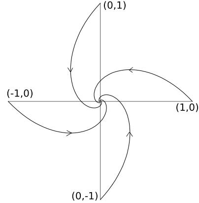
Demonstration in the case of a square.
The flies constantly form an EFGH square with the coordinates shown in the figure.
The collinearity of the speed vector at E with , results in , hence the differential equation of the curve: . By passing in polar coordinates the equation transforms into , hence the solution , with a = 1 into applying the initial condition.
A parameterization is therefore ; with this, the speed of the flies is , it decreases towards 0, and the time course is infinite, for a length (side of the starting square
).
With , the flies have a speed
constant equal to , for a travel time equal to 1.

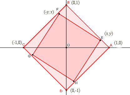
Figure : Elisabeth Busser

Case of a square, copied 4 times by symmetries
Case of an equilateral triangle, copied 7 times by symmetries

See also similar curves in 3D.

Did the anonymous Ivorian artist who designed this engraving think they were tracing pursuit curves?

next curve previous curve 2D curves 3D curves surfaces fractals polyhedra