Bifocal equation: 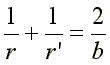 (with two foci F and F' at distance 2a from one another). Cartesian equation 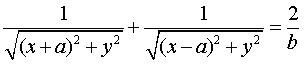: . Cartesian parametrization 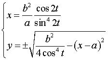: . Quadricircular biquartic.

Cayley ovals are the loci of the points on the plane for which the harmonic mean of the distances to two points, the foci, is constant (= b).

Therefore, they are the equipotential lines of the electrostatic potential created by two equal charges placed at the foci (or of the gravitational potential created by two identical masses).

Case b < a: the "oval" is composed of two egg-like shaped curves symmetrical about O.
Case e = 1 (b = a): the curve is shaped like an 8.
Case : the oval has the shape of an "ellipse" that is worn out at the summits of the minor axis.
Case : the oval finally has the shape of an oval, leaning towards a circular shape as e increases.

All this reminds strongly of the Cassinian ovals (who, themselves, are quartics); these two families can indeed be placed into the more general framework of loci of points on a plane for which the order p mean of the distances to 2 points is constant, with bifocal equation 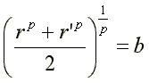  ; we can see above that Cassini and Cayley ovals are quite close; they can be distinguished by their tangents at O.
 

p = –	–  < p < -1	p = –1	–1 < p < 0
min ( r , r' ) = b
b = 0: foci, b = a: two tangent circles	b = 0: 2 points, b = a: eight	b = 0: 2 points, b = a: eight	b = 0: 2 points, b = a: eight
Arcs of circles centred on the foci		Cayley ovals

 

p = 0	0 < p < 1	p = 1
		r + r' = 2b
b = 0: 2 points, b = a: eight	b = 0: 2 points, b = a: eight	b = a: segment line
Cassinian oval		Ellipses

 

1 < p < 2	p = 2	2 < p < ¥	p = + ¥
	r2 + r'2 = 4b2		max ( r , r' ) = b
b = a: point O	b = a: point O	b = a: point O	b = a: point O
	Circles		Arcs of circles centred on the foci

Another generalisation consists in placing any charge at any point; the equipotential lines, with multifocal equation 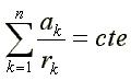 are called Cayley equipotential lines: they are, to Cayley ovals, what Cassinian curves are to Cassinian ovals.

Here are, for example, the equipotential lines (in red) with equation 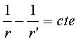 and the corresponding field lines (in blue) in the case of two particules of opposite charges.

For the limit case of these latter curves, when the poles come closer and closer to each other, see the curve of the dipole.

Of course, this can be generalised to curves with multifocal equation 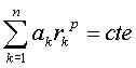 that result in Cayley equipotential lines when p = – 1. When p = – 2, we get the "equal-loudness" curves. They are the curves joining the points where the acoustic intensities, due to sound sources placed at the poles, are equal. See for example the isophonic curves for sources placed at the vertices of a triangle:

For other equipotential and field lines, see this page.

next curve

previous curve

2D curves

3D curves

surfaces

fractals

polyhedra

© Robert FERRÉOL 2023