Multipolar equation: 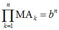. Complex equation: 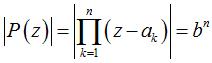, where P is a complex polynomial with distinct roots. Algebraic curve of degree 2n, n-circular curve. The Cassinian curves and the stelloids are the reciprocal images of the coordinate lines by the complex function f defined by 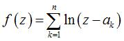. In the case of a regular polygon: Polar equation:  i.e., with ,  . Cartesian equation in this case: .

The Cassinian curves with n foci (or n poles) are the loci of the points on the plane for which the geometric mean of the distances to n points is constant.
When n = 2, we get the Cassini ovals.

The field lines of the magnetic field created by n parallel wires carrying currents of equal intensity in the same direction are, in any plane orthogonal to the wires, the Cassinian curves with foci the intersection points with the wires. The same is true for equipotential lines of the electrostatic field created by n uniformly charged parallel wires with identical charge.

I am looking for a picture of this experiment with.... iron fillings!

It can be shown that any simple closed curve can be approached as closely as wanted by a Cassinian curve, but with a number of poles that can be really large: Hilbert's lemniscate theorem (1897), find more details here.

When the poles are the vertices of a regular polygon with centre O and radius a and Ox passes by one of these vertices, then we get the polar equation given above.

When b < a, we get a curve composed of n ovals surrounding the vertices of the polygon.

When b = a (i. e. when the curve passes through O), we get a sinusoidal spiral with parameter n.

When b > a, we get a simple closed curve.
 

n = 3

n = 4

n = 5

The orthogonal trajectories of these curves, as b changes, are sinusoidal spirals with parameter -n, all similar to one another, with polar equation .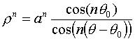

Cassinian curves can be generalised to weighted geometric means, in other words, to multipolar equations of the form: 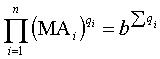. These curves can be physically obtained as magnetic field lines thanks to wires carrying distinct currents, or as electrostatic equipotential lines of wires with different charges.

For example, when n = 2 et , we get a pencil of circles for which the limiting points are the poles.

next curve

previous curve

2D curves

3D curves

surfaces

fractals

polyhedra

© Robert FERRÉOL 2017