ELASTIC CATENARY
| next curve | previous curve | 2D curves | 3D curves | surfaces | fractals | polyhedra |
ELASTIC CATENARY
| Curve studied by Finck and Bobillier in 1826. |
Differential equation: 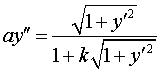 where
where Cartesian parametrization: 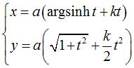 or
or 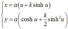 (
(Curvilinear abscissa: 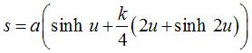 . .
Radius of curvature: Transcendental curve. |
The elastic catenary is the shape taken by an elastic,
homogeneous, infinitely thin, flexible, massive wire hanging from two points,
placed in a uniform gravitational field.
As for the ordinary catenary,
the equations of electrostatics give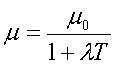 where l is the elasticicty coefficient
of the wire and
where l is the elasticicty coefficient
of the wire and It can be integrated to 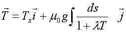 therefore
 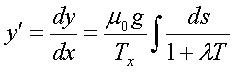 (1); it also shows that the horizontal tension
 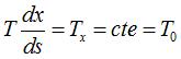 so that, by differentiating (1), we get the differential equation of the
elastic catenary:
so that, by differentiating (1), we get the differential equation of the
elastic catenary: 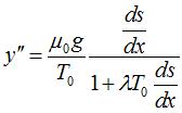
i.e., with  and .
and . |
 |
This equation, with no x nor y, can be
written as 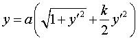 ,
hence the above parametrization when y' is taken as a parameter. ,
hence the above parametrization when y' is taken as a parameter.
With the above notations, if the wire is described when u ranges between -U and U, the value of U can be implicitly calculated by the formula |
 |
On the left, an animation showing the various positions
of the elastic catenary, for an elasticity coefficient growing from 0,
and for a wire with fixed mass and given length at rest. The curve is higher
than the classic catenary.
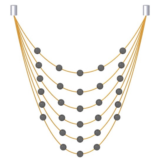
It can be noticed that the total extension is basically proportional to the elasticity. On the right, equidistant positions have been marked by circles on the initial catenary. Note that the horizontal position stays approximately the same during the extension. |
 |
If we forget the initial physical problem, by setting
b=ka, we obtain the equations 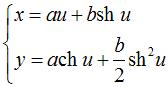 which
give the ordinary chain for b = 0, and the parabola x²
= 2by for a = 0. which
give the ordinary chain for b = 0, and the parabola x²
= 2by for a = 0.
The elastic chain therefore provides all the positions intermediaries between the ordinary chain and the parabola. Opposite, an illustration of this fact (the catenary is in blue and the parabola in green). |
 |
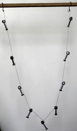 |
Experiment: the bolts were equidistant on the elastic wire at rest. |
 |
| next curve | previous curve | 2D curves | 3D curves | surfaces | fractals | polyhedra |
© Robert FERRÉOL 2017