
-1< k < 0: pseudo-sinusoid
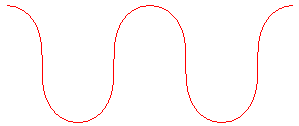
k = 0
right lintearia
| next curve | previous curve | 2D curves | 3D curves | surfaces | fractals | polyhedra |
ELASTIC CURVE, or ELASTICA, or ELASTIC ROD

-1< k < 0: pseudo-sinusoid |

k = 0 right lintearia |
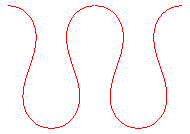 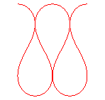 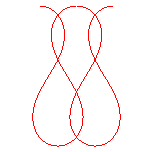 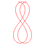
. 0< k < k1 = 0.65222.... |
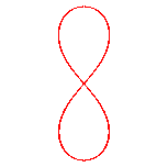
k = k1 = 0.65222....: pseudo-lemniscate |
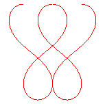 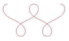
k1< k < -1 |

k = 1 : convict curve |
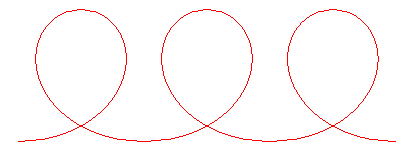 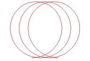
k > 1: pseudo-trochoid |
| Curve studied by Jacques Bernoulli in 1691 who named
it elastica, by Euler in 1744, and Poisson in 1833.
Other names: lintearia, radioid with curvature proportional to the abscissa. See on this page of Alain Esculier a program to trace this curve. |
The elastic curves are the plane curves the curvature
of which is, at all points, proportional to the distance to a fixed line,
called the directrix.
| With the directrix as the y axis, the condition
can be written Differential equation: (1) that can be integrated into With Curvilinear abscissa: |
For -1 < k < 1 (figure with k = 1/ 2: tangential angle at the origin equal to - 30 °)
If we use the parametrization:
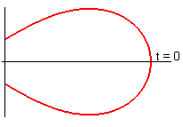 |
If we use the explicit expression:
|
| Cartesian parametrization: With |
Here, Cartesian equation: with |
For k = 1:
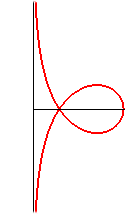 |
The integral is no longer elliptic and we have
the parametrization:
|
For k > 1:
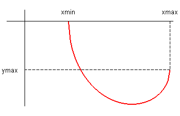 |
Cartesian equation: where with |
According to the Young-Laplace
equation, the profile of a rectangular tarpaulin full of water is an
elastic curve (the curvature of the tarpaulin being proportional to the
distance to the surface of the liquid), hence the name lintearia.
We also find this curve as the trajectory of a torpedo
the rudder of which turn with an angle proportional to the depth.
But the elastic curve is also the solution to the following
calculus of variations problem: finding, among all the curve with given
length, that which minimises the integral of the square of the curvature ;
in other words, it is the curve that minimises the variance of the oscillations
of the tangent with respect to a fixed direction. It is the reason why
it can be found in many natural phenomena.
 |
 |
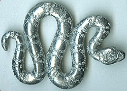 |
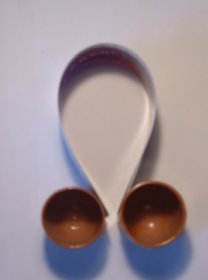
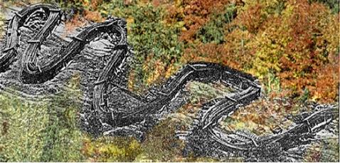
| An elastic blade constrained to assume the shape of an elastic curve (hence the name) | During this railway accident, the tracks assumed the shaped of an elastic curve, called "buckling coil" by physicists. | The undulations of snakes, minimising the curvature, have the shape of elastic curves. |
 |
The meanders of rivers take the shape of elastic curves
(see also the meander curve)
Here, the meanders of the Somme river. |
Because of the characteristic property of minimising the curvature, the elastic curve is sometimes used for the layout of roads between two linear portions, hence the name of radioid.
It is also a solution to this other calculus of variations
problem: finding a curve of given length joining two given points A
and B, for which the rotation around a line (D) coplanar
with the line (AB) generates a solid with maximal volume (in other
words, maximal
for constant
).
And it is also characterised by the fact that when a point
M
describes it at constant speed, the tangent oscillates around
M
the same way a simple pendulum would oscillate around the parallel to the
directrix passing by M (cf. the formula ).
It is the reason why the elastic curve is very similar, for values of k between 1 and 1 to the meander curve (the tangent of which has sinusoidal oscillations), and why they are often mixed up.
See on this German site a very beautiful animation of a generalisation of this curve.
See also the hanging drop of water, generalisation to space of the elastic curve.
The curves such that the curvature is proportional to
the distance to a fixed point (instead of a line) are studied on
the page of the Norwich spiral;
we find, in particular, the lemniscate
of Bernoulli.
The curves such that the curvature is proportional to
the curvilinear abscissa are the clothoids.
The curves such that the curvature is proportional to
the distance to the intersection point between the normal and a fixed
line are studied here.
REMARK: if, in the differential equation ,
the exponent 3/2 is replaced by 1/2, we get the skipping
rope curve.


| next curve | previous curve | 2D curves | 3D curves | surfaces | fractals | polyhedra |
© Robert FERRÉOL 2017