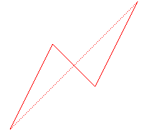
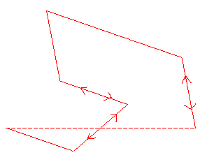
et son transformé
loi : F=FGF
G=GGG
cantor(A, (2*A+B)/3, n-1),cantor((A+2*B)/3, B, n-1)
fi end:plot([cantor([0,0],[1,0],4)],axes=none,color=red);
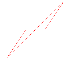
if n=0 then [a,b],[c,d] else
escalieroblique(a, b, (2*a+c)/3, (b+d)/2, n-1),
escalieroblique((a+2*c)/3, (b+d)/2, c, d, n-1)
fi end:
plot([escalieroblique(0,0,1,1,6)],axes=none,color=red);
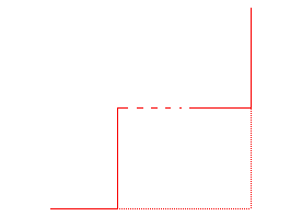
if n=0 then [a,b],[c,b],[c,d] else
escalierdroit(a, b, (2*a+c)/3, (b+d)/2, n-1),
escalierdroit((a+2*c)/3, (b+d)/2, c, d, n-1)
fi end:
plot([escalierdroit(0,0,1,1,6)],axes=none,color=red);
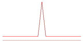
(t = 1/2 : escalier de Cantor,
t =2/3 : courbe de Bolzano-Lebesgue proprement dite)
if n=0 then [a,b],[c,d] else
bolzaleb(a,b,(2*a+c)/3,(1-t)*b+t*d,t,n-1),
bolzaleb((2*a+c)/3,(1-t)*b+t*d,(a+2*c)/3,t*b+(1-t)*d,t,n-1),
bolzaleb((a+2*c)/3,t*b+(1-t)*d,c,d,t,n-1)
fi end:
plot([bolzaleb(0,0,1,1,2/3,5)],axes=none,color=red);
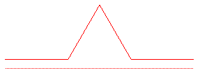
| numéro du segment | 1 | 2 | 3 | 4 |
| longueur | 1/3 | 1/3 | 1/3 | 1/3 |
| angle avec le segment de départ | 0° | 60° | -60° | 0° |
loi :
F=F-F++F-F
avec t1 = t2= 60°
if n=0 then A else
koch(A, (2*A+B)/3, n-1),
koch((2*A+B)/3, (A+B)/2+I*(B-A)/sqrt(3)/2 ,n-1),
koch((A+B)/2+I*(B-A)/sqrt(3)/2, (A+2*B)/3, n-1),
koch((A+2*B)/3, B, n-1)
fi end:
complexplot([koch(0,1,4),1],axes=none,color=red,scaling=constrained);
(avec 1/4 £ t £ 1/2 ;
t = 1/3 : courbe de Koch,
t =1/2 : courbe de Césaro)
| numéro du segment | 1 | 2 | 3 | 4 |
| longueur | 1/2 | 1/2 | 1/2 | 1/2 |
| angle avec le segment de départ | 0° | 90° | -90° | 0° |
if n=0 then A else
poumon(A, (1-t)*A+t*B, t, n-1),
poumon((1-t)*A+t*B, (A+B)/2+I*(B-A)*sqrt(t-1/4), t, n-1),
poumon((A+B)/2+I*(B-A)*sqrt(t-1/4), t*A+(1-t)*B, t, n-1),
poumon(t*A+(1-t)*B, B, t, n-1)
fi end:
complexplot([poumon(0,1,0.45,4),1],axes=none,color=red,scaling=constrained);
| numéro du segment | 1 | 2 |
| longueur | 1/Ö2 | 1/Ö2 |
| angle avec le segment de départ | 45° | -45° |
loi :
F=-F++F
avec t = 45°
if n=0 then A else
c(A, (A+B)/2+I*(B-A)/2, n-1),
c((A+B)/2+I*(B-A)/2, B, n-1)
fi end:
complexplot([c(0,1,8),1],axes=none,color=red,scaling=constrained);
| numéro du segment | 1 | 2 |
| longueur | 1/Ö2 | 1/Ö2 |
| angle avec le segment de départ | 45° | -45° |
if n=0 then [A,B] else
dragon((A+B)/2+I*(B-A)/2, A, n-1),
dragon((A+B)/2+I*(B-A)/2, B, n-1)
fi end:
complexplot([dragon(0,1,8)],axes=none,color=red,scaling=constrained);
(deuxième type)
| numéro du segment | 1 | 2 | 3 | 4 | 5 | 6 | 7 | 8 | 9 |
| longueur | 1/3 | 1/3 | 1/3 | 1/3 | 1/3 | 1/3 | 1/3 | 1/3 | 1/3 |
| angle avec le segment de départ | 0° | 90° | 0° | -90° | 180° | -90° | 0° | 90° | 0° |
loi :
F=F-F+F+F+F
-F-F-F+F
peano(A,(2*A+B)/3,n-1),
peano((2*A+B)/3,(2*A+B)/3+I*(B-A)/3,n-1),
peano((2*A+B)/3+I*(B-A)/3,(A+2*B)/3+I*(B-A)/3,n-1),
peano((A+2*B)/3+I*(B-A)/3,(A+2*B)/3,n-1),
peano((A+2*B)/3,(2*A+B)/3,n-1),
peano((2*A+B)/3,(2*A+B)/3-I*(B-A)/3,n-1),
peano((2*A+B)/3-I*(B-A)/3,(A+2*B)/3-I*(B-A)/3,n-1),
peano((A+2*B)/3-I*(B-A)/3,(A+2*B)/3,n-1),
peano((A+2*B)/3,B,n-1)
fi end:
complexplot([peano(0,1+I,3),1+I]),axes=none,color=red,scaling=constrained);
(premier type)
peanosierp(A,(2*A+B)/3,n-1),
peanosierp((2*A+B)/3,(2*A+B)/3+I*(B-A)/3,n-1),
peanosierp((2*A+B)/3+I*(B-A)/3,(A+2*B)/3+I*(B-A)/3,n-1),
peanosierp((A+2*B)/3+I*(B-A)/3,(A+2*B)/3,n-1),
peanosierp((2*A+B)/3,(2*A+B)/3-I*(B-A)/3,n-1),
peanosierp((2*A+B)/3-I*(B-A)/3,(A+2*B)/3-I*(B-A)/3,n-1),
peanosierp((A+2*B)/3-I*(B-A)/3,(A+2*B)/3,n-1),
peanosierp((A+2*B)/3,B,n-1)
fi end:
complexplot([peanosierp(0,1+I,3)],axes=none,color=red,scaling=constrained);
| numéro du segment | 1 | 2 | 3 |
| longueur | 1/2 | 1/2 | 1/2 |
| angle avec le segment de départ | 60° | 0° | 60° |
if n=0 then [A,B] else
sierpinski((3*A+B)/4+I*(B-A)*sqrt(3)/4,A,n-1),
sierpinski((3*A+B)/4+I*(B-A)*sqrt(3)/4,
(A+3*B)/4+I*(B-A)*sqrt(3)/4,n-1),
sierpinski(B,(A+3*B)/4+I*(B-A)*sqrt(3)/4,n-1)
fi end:
complexplot([sierpinski(0,1,6)],axes=none,color=red,scaling=constrained);
(premier type)
Y = +XFYFYFX+
if n=0 then (3*A+B)/4+e*I*(B-A)/4,(3*A+B)/4+3*e*I*(B-A)/4,
(A+3*B)/4+3*I*e*(B-A)/4,(A+3*B)/4+e*I*(B-A)/4 else
hilbert(A,A+e*I*(B-A)/2,n-1,-e),
hilbert(A+e*I*(B-A)/2,(A+B)/2+e*I*(B-A)/2,n-1,e),
hilbert((A+B)/2+e*I*(B-A)/2,B+e*I*(B-A)/2,n-1,e),
hilbert(B+e*I*(B-A)/2,B,n-1,-e)
fi end:
complexplot([hilbert(0,1,2,1)]),axes=none,color=red,scaling=constrained);
(deuxième type)

if n=0 then [A,B] else
hilbert2(A+I*(B-A)/2,A,n-1),
hilbert2(A+I*(B-A)/2,(A+B)/2+I*(B-A)/2,n-1),
hilbert2((A+B)/2+I*(B-A)/2,B+I*(B-A)/2,n-1),
hilbert2(B,B+I*(B-A)/2,n-1)
fi end:
complexplot([hilbert2(0,1,4)]),axes=none,color=red,scaling=constrained);
départ : A
Loi :
A =B-A-B,
B= A+B+A
angle : 60º
| numéro du segment | 1 | 2 | 3 | 4 | 5 | 6 | 7 | 8 |
| longueur | 1/3 | 1/3 | 1/3 | 1/3 | 1/3 | 1/3 | 1/3 | 1/3 |
| angle avec le segment de départ | 0° | 90° | 0° | -90° | -90° | 0° | 90° | 0° |
if n=0 then A else
mink(A,(3*A+B)/4,n-1),mink((3*A+B)/4,(3*A+B)/4+I*(B-A)/4,n-1),
mink((3*A+B)/4+I*(B-A)/4,(A+B)/2+I*(B-A)/4,n-1),mink((A+B)/2+I*(B-A)/4,(A+B)/2,n-1),
mink((A+B)/2,(A+B)/2-I*(B-A)/4,n-1),mink((B+A)/2-I*(B-A)/4,(A+3*B)/4-I*(B-A)/4,n-1),
mink((3*B+A)/4-I*(B-A)/4,(A+3*B)/4,n-1),mink((A+3*B)/4,B,n-1)
fi end:
complexplot([mink(0,1,1),1],axes=none,color=red,scaling=constrained);
| numéro du segment | 1 | 2 | 3 | 4 | 5 | 6 | 7 |
| longueur | 1/Ö7 | 1/Ö7 | 1/Ö7 | 1/Ö7 | 1/Ö7 | 1/Ö7 | 1/Ö7 |
| angle avec le segment de départ | 0-a° | 60-a° | 180-a° | 120-a° | -a° | -a° | -60-a° |
u:=evalf(exp(I*Pi/3)):v:=evalf((B-A)*exp(-I*arctan(sqrt(3)/5))/sqrt(7)):
P:=A+v:Q:=P+u*v:R:=Q-v:S:=R+u^2*v:T:=S+v:U:=T+v:
if n=0 then[A,B] else
gosper(A,P,n-1),
gosper(Q,P,n-1),
gosper(R,Q,n-1),
gosper(R,S,n-1),
gosper(S,T,n-1),
gosper(T,U,n-1),
gosper(B,U,n-1)
fi end:
complexplot([gosper(0,1,4)],axes=none,color=red,scaling=constrained);
local k,M;
k:=nops(L):M:=evalf([seq(L[q]*exp(t[q]*I),q=1..k)]);
if n=0 then [A,B] else
[A,B],seq(arbre(B,B+M[q]*(B-A),L,t,n-1),q=1..k)
fi end:
complexplot([arbre(0,I,[0.7,0.7],[Pi/9,-2*Pi/9],7)],
axes=none,color=COLOR(RGB,0.55,0.2,0),scaling=constrained);
local k,M;
k:=nops(L):M:=evalf([seq(L[q]*exp(t[q]*I),q=1..k)]);
if n=0 then [A,B] else [A,B],
fougere(B,B+M[1]*(B-A),L,t,n-1),
fougere(B,B+M[2]*(B-A),L,subsop(1=-t[1],t),n-1),
fougere(B,B+M[3]*(B-A),L,t,n-1)
fi end:
complexplot([fougere(0,I,[0.85,0.33,0.33],[0.05,0.4*Pi,-0.4*Pi],5)]),
axes=none,color=COLOR(RGB,0.1,0.9,0),scaling=constrained);