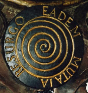
Curve studied by Descartes and Torricelli in 1638, then by Jacques Bernoulli (1654-1705). Other names: equiangular spiral, Bernoulli spiral, spira mirabilis; the name "logarithmic spiral" was given by Varignon. Jacques Bernoulli had a logarithmic spiral engraved on its gravestone in the Basel Munster, with the epigraph: eadem mutata resurgo, "although changed (mutata), I arise (resurgo) the same (eadem)". Nonetheless, the engraver traced an Archimedean spiral...

 

Polar equation: , k being the cotangent of the constant polar tangential angle: . Complex parametrization: . Transcendental curve. Curvilinear abscissa and intrinsic equation 2: 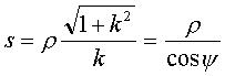, s being counted from the asymptotic point O. Radius of curvature: 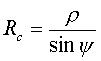.  Intrinsic equation 1: . Intrinsic equation 2: 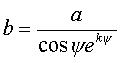 (with ). Pedal equation: .

The logarithmic spiral can be defined as
    - the curve the polar tangential angle of which  remains constant (different from a right angle)
    - the curve the curvature of which is inversely proportional to the curvilinear abscissa
    - the curve the radius of curvature of which is inversely proportional to (and greater than) the radius vector ( with l > 1)
Therefore, the logarithmic spirals with centre O are the trajectories at angle. of the pencil of lines issued from O.

The logarithmic spiral is also the stereographic projection from the south pole of the rhumb lines of the spheres with centre O, forming an angle  with the meridians (since the stereographic projection is a conformal map).

Finally, it is the planar expansion of an helix of a cone of revolution.

The logarithmic spiral has an exceptional stability with respect to the classic geometrical transformations:

    - any rotation with centre O and angle  of the spiral amounts to a homothety with same centre and ratio , which in turn amounts to the identity if .

eadem mutata resurgo... Rotation equals homothety!

Homothety equals identity!

   Note that the property "eadem mutata resurgo" is characteristic of this curve: any continuous curve which, when turned by an angle , is equal to its homothetic image with ratio (for any angle ) is a logarithmic spiral with k = - ln. For an Archimedean spiral, a rotation is completely different from a homothety!

    - any inversion with centre O amounts to a reflection about an axis passing by O.
    - its evolute is a logarithmic spiral with same centre and same angle(and, besides, the limit of the n-th evolute of any curve is a logarithmic spiral).

     - its caustics by reflexion or diffraction, when the light source is at O, are logarithmic spirals.

    - the mating gear associated to a gear shaped like an logarithmic spiral is an isometric logarithmic spiral.

When a logarithmic spiral rolls on a line, the asymptotic point describes another line:

The logarithmic spiral is a solution to the three following physical problems:

    1) The force centred on O that makes a point in space describe a logarithmic spiral is proportional to 1/r³ (this force, according to the Binet formula, is proportional to  which, here, is equal to , with u = 1/r).
    2)  the curve (called brachistochrone) that minimises the travel time of a point moving freely along this curve, when it is itself turning around a fixed centre O at constant speed, in the case where the speed of the moving point vanishes at O, is a logarithmic spiral.

    3) A particle of mass m₁ and charge q placed in a uniform magnetic field of intensity B with a speed v₀ perpendicular to the field describes a logarithmic spiral with  and .

see: perso.libertysurf.fr/hdehaan/mecanique/M6/M6_2/M6_2_cadre.htm
 
 

If u is a complex number different from 0, then the image points of the geometric sequence  with common ratio u are located on an exact logarithmic spiral, with parameter . Opposite, u = 1+i/4.

In the same way, any sequence points of polar coordinates  such that the  are in geometric progression with common ratio a and the  are in arithmetic progression with common difference b describes a logarithmic spiral with k = ln a / b. For example, on the opposite figure, the points with polar coordinates ((1,1)k  ; (k+2l)p/n) were traced, in blue if l is even, in red otherwise. These points are placed in a quincunx pattern at the intersection between concentric circles with radii in geometric progression and concurrent lines; but they are also located on the logarithmic spirals with equation , hence the nice visual effect.

The tablecloth in my living room

 

Here, the same spirals, but coloured in triangles in the style of this mosaic which adorned a Roman villa in Corinth in the 2nd century AD.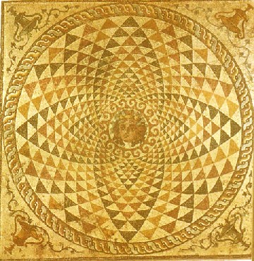

 

Furthermore, as it could be noticed on the previous figures, the spirals  and  form two orthogonal lattices.

 

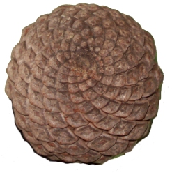
Phyllotaxis The scales of pine cones develop on a logarithmic spiral in such a way that the angular difference (in relation to the centre) between two consecutive scales is the golden angle equal to  where  is the golden ratio; the scales can then be classified into secondary spirals, the cardinality of a certain kind always being a Fibonacci number; here, there are 13 red spirals and 8 green ones.

 

View of points of polar coordinates  with r = 1 005, located on the spiral , for N ranging from 0 to 100, simulating the scales. The black angle connecting the first two scales is therefore equal to the golden angle. red secondary spirals and  secondary green spirals appear, which rather models the sunflower florets. On the view secondary spirals. On the picture where the scales are indicated with the appearance number, we note that the k-th secondary spiral is associated with  is formed of the points  satisfying N = k + a multiple of , for k ranging from 0 to ; for example, the first red spiral connects scales whose number is multiple of 21. The scales of the k-th secondary spiral associated with 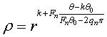 are located on the logarithmic spiral of polar equation  where  is the integer closest to , ie , seen the links between the Fibonacci sequence and the golden ratio ( is the polar angle between two successive scales of a secondary spiral). Note: the angle between two red and green spirals that intersect is constant but not related to the golden angle as we sometimes see written, since it depends on the value of r!
If we increase the ratio r to 1.02, it is rather the 8 =  red spirals associated with  and the 13 =  green spirals associated with , which are visible naturally, as for the pine cone; on the second figure are drawn the 34 =  red spirals associated with  and  the 55 =  green spirals associated with , again with r = 1.005. These secondary spirals associated with the Fibonacci numbers appear visually because multiplying the golden angle by the terms of the Fibonacci sequence yields results the moduli of which approach zero for large n: we can see clearly in the figure where the scales are indicated with their number of appearance that the fibonaccian scales 3, 5, 8, 13, 21, 34, 55, 89 are close to the x axis. On this page, we can test different angles of rotation between two sunflower florets and note that the arrangement of the florets is optimal in the case of the golden angle.

If we consider a sequence of concurrent lines D₁, D₂, .... each of them forming an angle e with the next one, and so that if, starting from M₁ on D₁, M₂ on D₂ is defined so that the angle between D₁ and M₁M₂ is equal to , and M₃, M₄, ... are defined in the same way, then the moduli of the points M_n are in geometric progression with common ratio  and their arguments are in arithmetic progression with common difference e, and thus are on a logarithmic spiral with 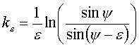; it can be checked that  goes indeed to cot  as  goes to 0, so that the spiral corresponding to goes to the logarithmic spiral with k = cot .
 

here, y = 100°, e = p/10.

here, y = 100°, e = p/50.

REMARK: when  = 90°, M_i+1 is defined so that M_i is its orthogonal projection on D_i (careful not to mistake it with the Theodore spiral which is an approximate Archimedean spiral).

Another approximate construction consists in taking arcs of circles with constant angles  and radii in geometric progression with common ratio , with tangential connection.
For a very beautiful special case, see the golden spiral.
The spiral traced on a cone which is projected on a logarithmic spiral is the conical helix.

See also the spiral of the rotating rod and the mutual pursuit curves.

next curve

previous curve

2D curves

3D curves

surfaces

fractals

polyhedra

© Robert FERRÉOL 2019