A Cartesian oval is the locus of the points M for which the distances MF and MF' to two fixed points satisfy a relation of the type: , with  (the limit cases of the ellipse and the hyperbola are therefore excluded).
Remark: the curve is not empty iff  and .

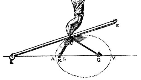
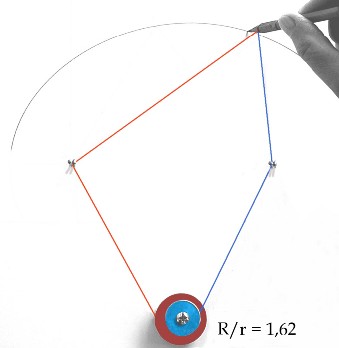
Find above a mechanical construction of the Cartesian oval, in the case where v/u = 2, construction the can be generalised (theoretically), on the condition to wrap the wire around the pulleys enough, to the cases where v/u is a nonnegative rational. On the right, the illustration is due to Descartes himself.
 

Another mechanical construction, due to J. Hammond (1878). The two pulleys are integral, their common axis has an arbitrary position in the plane of the figure, only the ratio of their radius equal to v/u matters. Once the foci have been chosen, two threads are wound, in opposite directions, on the pulleys. The tip of the pencil, fixed relative to the wire, is attached to the other end of each of the two wires. Diagrams of Jean Lochet.

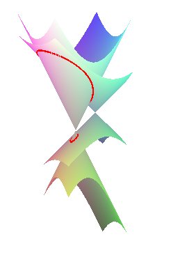
A construction in space: the Cartesian ovals are the projections of the intersections between two cones of revolution with parallel axes on a plane perpendicular to these axes (Quételet theorem). More precisely, the cone  and the cone  have an intersection that is projected on the Cartesian ovals: . On the right, geometric proof, for cones with vertices S and S' and half angles a and a': .

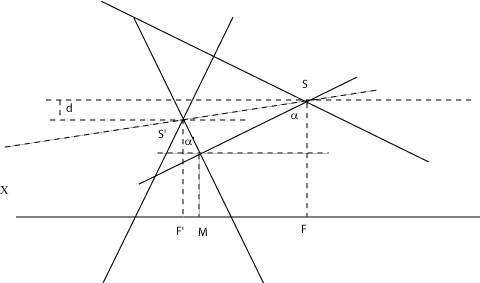This construction is the source of a planar construction, due to Chasles, whose 3D origin can be forgotten. Cut the two cones by a plane (P0) perpendicular to the axes. This gives two circles (C) and (C') with centres F et F'; the line joining the vertices S and S' of the two cones cuts (P0) at the point X, and X, F, and F' are aligned. Any plane (P) passing by F and F' cuts (P0) on a line (D) passing by X. This plane (P) cuts the two cones along two generatrices, which themselves intersect at a point in the intersection of the two cones. When projecting, the line joining F to an intersection point between (C) and (D) and the line joining F' to an intersection point between (C') and (D) intersect at a point M on the Cartesian oval, projection of the intersection of the two cones (and since there are two intersection points for each circle, this constructs 4 points M). When the line (D) turns around X, each of the 4 points M describes a half Cartesian oval. This way we get two conjugate Cartesian ovals (see the definition later). Origin: [Zwikker, p. 124]	Proof without the space: the Menelaus theorem in the triangle MFF' for the transversal line (D) gives , hence
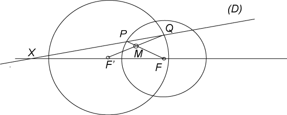
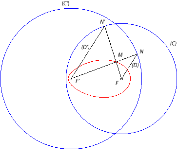
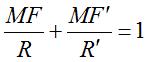Given two circles (C) and (C') with centres F and F' and radii R and R' greater than or equal to FF', we get the Cartesian oval  by drawing variable parallel lines (D) and (D') passing by F and F', the first one cutting (C') at N and the second one cutting (C) at N', on the side of (FF'). The intersection M between (FN') and (F'N) describes the Cartesian oval. Proof: Using Thales' theorem, we have MF.MF' = MN. MN'=(R'-MF')(R-MF) hence R' MF +R MF' = RR'.  We get this way all the non-empty ovals , with u,v,c > 0 (). This construction is a generalisation of the construction of the ellipse with an antiparallelogram (case R = R').
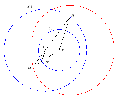
If we follow the previous construction but take the intersection points N between (D) and (C') and N'' of (D') and (C) on either sides of (FF'), the intersection point M' between (FN" and (F'N) describes now the conjugate Cartesian oval to the previous one, with equation 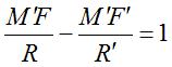(case R' > R). Proof: Using Thales' theorem, we have M'F.M'F' = M'N. M'N"=(R'+M'F')(-R+M'F) hence R' M'F -R M'F' = RR'.

 

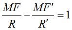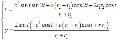With R = 2a, R'=2b, F=(0,c), F'=(– c,0), the construction above gives the following parametrizations  of the ovals  and , with , : and 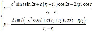. Remark: the case R and R' > FF' studied here corresponds to that where the two foci are inside the oval; the other cases give the third focus (see after).

 

The tangent at M to the oval is orthogonal to the vector 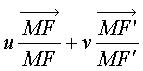.  Then, if  and  are the angles formed by the normal and the segment lines MF and MF' at M, we have the relation . From this we deduce the property that motivated the study of these curves by Descartes: if the external part of a Cartesian oval containing F has a refraction index n1  and the internal part containing F' has an index n2, with , the light rays emitted by F and refracted by the oval converge to F' (on the condition that [MF] be entirely outside and [MF’] inside). This is the origin of the name aplanatic curve. This property can also be found by using that the optical path length  is constant.

Figure with the oval MF+3MF'=2FF'. Therefore, here, .

More generally, the caustic by refraction of the oval for the light source F and the ratio u/v is the focus F': the Cartesian ovals are the curves for which a caustic by refraction is reduced to a point.

The associated complete Cartesian oval is the set with bifocal equation: .
Among the four curves obtained by these double signs, only two are not empty, and theese two ovals are said to be conjugate.
It can be proved that the Cartesian oval has a third focus, aligned with the first two, such that the bifocal equations with the two new couples of foci are still of the same type.
These relations between these foci and the equation are given below. The foci are renamed "A, B, C", to correspond to . These are the notations we will use from now on.
 

If  are the three foci of the complete oval, with : Equivalent bifocal equations of the external oval: 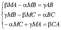. Equivalent bifocal equations of the internal oval: 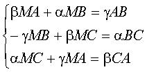. For the oval 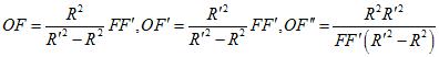, the point O and the focus F'' are defined by:
Animation in the case where ; the focus B moves from A to C; the two limit cases are limaçons of Pascal.

Cartesian equation of the complete oval in the frame : , where  are the elementary symmetric polynomials of . Abscissas of the 4 vertices:  (external oval) and  (internal oval). Polar equation of the complete oval in the frame :  where , , . Similar equations obtained by permutation of  in the frames  and . Cartesian equation in : . Bicircular quartic, elliptic in the case of a true oval.

The polar equation  shows that complete Cartesian ovals are anallagmatic: they are the cyclic curves with initial curve a circle. In other words, they are Cartesian curves. More precisely, they are the Cartesian curves for which the three real foci are aligned.
For the focus A, the initial circle is the circle with centre O and radius  where, the directrix circle, the circle with centre A and radius  (for the other two foci, the definitions are obtained by permutation).

When the three foci are different points, the oval is called true oval. It then has three different cyclic definitions: View of the 3 cyclic generations of the same complete Cartesian oval; the black circles are centred on the initial circle (in blue), itself centred on O, and are orthogonal (or pseudo-orthogonal for the one on the right) to the directrix circle (in green), centred on one of the foci A, B or C; here we took a = 1, b = 2, g = 3.

The six directrix and initial circles.

When the 3 foci coincide (), the oval is a cardioid (but it loses its bifocal definitions).
When only two of the three foci coincide, we get a limaçon of Pascal:
     - when A = B, we get the elliptic limaçon:  (in ), with bifocal equation: , which has two cyclic generations, among which only one has a zero power.
 

generation with zero power (circles passing by A and centred on the initial circle)

 - when B = C, we get the hyperbolic limaçon:  (in ), with bifocal equation  for the external loop, and  for the internal loop, which has two cyclic generations, among which only one has a zero power.
 

generation with zero power (circles passing by B and centred on the initial circle)

The complete Cartesian ovals can also be defined as the anticaustics of circles (the limaçons of Pascal being obtained when the light source is on the circle). The evolute of complete Cartesian ovals are therefore caustics by refraction of circles.

Here are the geometrical loci that give Cartesian ovals:

1) Locus of a point for which the "algebraic distances" to two fixed circles with different radii have a constant ratio different from ± 1 (in which case we would get the bifocal conics). The "algebraic distance" of a point to a circle is its distance to the centre minus the radius. The Cartesian ovals are therefore the dividing lines of two circles.
 

Dividing lines of two circles, defined by . In green for k > 1, in blue for 0 < k < 1, in red for k = 1 (branch of a hyperbola, perpendicular bisector of the two circles).

 

2) Given 3 aligned points F, G, H, locus of the vertex M of a triangle LMN such that the sides (NM), (ML), (LN) contain, respectively, F,G,H, when [ML] and [MN] have given fixed lengths (apply Menelaus theorem in the triangle MFG).

The Cartesian ovals are also found in the Bélidor drawbridge curve.

Another property of these very rich curves: the images of the lines parallel to the axes by an elliptic function P of Weierstrass with real period w₁ and imaginary period w₂ are Cartesian ovals.

next curve

previous curve

2D curves

3D curves

surfaces

fractals

polyhedra

© Robert FERRÉOL  2023